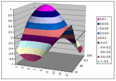
How to Create a 3d Chart in Excel

Microsoft Excel is one of the most widely used software. It is an important component of Microsoft Office which has been released by Microsoft in different versions. You can easily store multi-dimensional data in Microsoft Excel. It offers many tools by which you can interpret and analyse the data according to your requirement.
Microsoft Excel 2007 provides you the option of making 3D charts. 3D charts are more presentable and make data analysis easier. It is not very difficult to create 3D charts in Excel. All you need is to follow some basic guidelines.
Things Required:
– Computer
– Microsoft Excel 2007
Instructions
-
1
First of all, you have to open Microsoft Excel on your computer. You can simply open it by searching from the list of applications given under Microsoft Office in programmes. You will have to enter the necessary data in order to create a 3D chart.To create your chart you can use an existing data or you can simply enter new data in a workbook.
-
2
Select the data and click on insert button given in the menu bar. You will see many options on your screen. Select the option of charts and you will see different categories of charts.
Select the category of 3D chart. Click on the blank area of the chart and click on the ‘Format’ tab in order to display the design options. You can see a lot of shapes and styles in the formatting option. Choose your favourite chart option in 3D Format and click on it. -
3
After that, you have to set the width and height of the bevel of the chart. Click on ‘Bevel’ section to open the ‘Format Chart Area’ option. Then, choose your desired colour, contour and size of your chart. You can also select your favourite angle of lighting, type of lighting and material for your chart from the ‘Surface’ section of the option box.
-
4
Just click on ‘Close’ button in order to close the ‘Format Chart Area’ box. Return to the chart and see whether the chart contains your desired settings or not. If not, go to the ‘Format Chart Area’ again to make the necessary changes. Just save your workbook by clicking on ‘Save’ or ‘Save As’ option.


