How to Calculate Compound Interest Using Excel
Calculation of compound interest is comparatively complicated than doing the same for simple interest. If you want to calculate your compound interest, there are different ways for doing that. You can do it manually with the help of a small formula, where all you have to do is insert the values and press the buttons of calculator a few times and the result will be in front of you. Nevertheless, if it is more of a daily routine for you and you want to be save time then Excel is a better choice.
Instructions
-
1
Realise the need
It is important that you should understand the need to calculate compound interest using Microsoft Excel. Calculating the interest using Excel is very different than doing the same task manually. With the help of Excel, you can perform the same task in a much quicker time and all you have to do is insert values in the designated columns, the rest is the task of Excel. -
2
Know the benefits
Calculating the compound interest on Excel provides numerous benefits to an individual. By using the Excel worksheet for calculation of compound interest, an individual can not only saves time and improves efficiency, but it also helps in keeping the record at a safe place. Not to mention, the easy access to calculations and convenience of knowing the figures at a glimpse is very beneficial. -
3
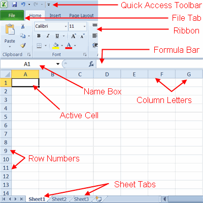
Open Excel file
You must open a new Excel document from ‘All Programs’ in the ‘Start menu’. If you do not have excel installed into your system, you should buy the DVD of Microsoft Office from a store and follow the instructions to install it on your computer. -
4
Give headings
After you have opened your document, you will be displayed with a huge number of rows and columns. Do not get confused with these big numbers and there is no need to scroll down, just stay on the top of the page. It is important that you give headings to the columns for your own convenience and better understanding.
A - Amount Invested
B - Yearly Percentage Rate
C - Number of Times Compounded Annually
D - Number of Years
F - Future Value -
5
Insert Values
Now you should insert the values into nominated columns. If you have taken $2000 for 2 years at a quarterly rate of 3% then
A - 2000
B - 0.03
C – 4
D – 2
You must insert the following function into row F: =A2*((1+B2/C2)^(C2*D2)).
